Modeling

Decision of a modeling method

At the beginning of the modeling process, the user needs to make an individual decision regarding whether to perform de novo modeling or not. Alternatively, a knowledge-based modeling method is available as an option. It is important to consider the available input when making this decision. In the case of de novo modeling, an RNA sequence is crucial. De novo modeling is beneficial when no pre-existing structures are found in databases or when modeling an ensemble of states is desired. On the other hand, knowledge-based modeling can be applied when considering tertiary structures that cannot be generated through de novo modeling. It is also useful when there are already resolved structures in databases that require minor changes in sequence or structure. This approach can even be used to retrospectively edit de novo models in order to generate structures that were not represented in the initial modeling process. In all cases, a clear understanding of the desired structure and its essential features is necessary when using the knowledge-based approach.

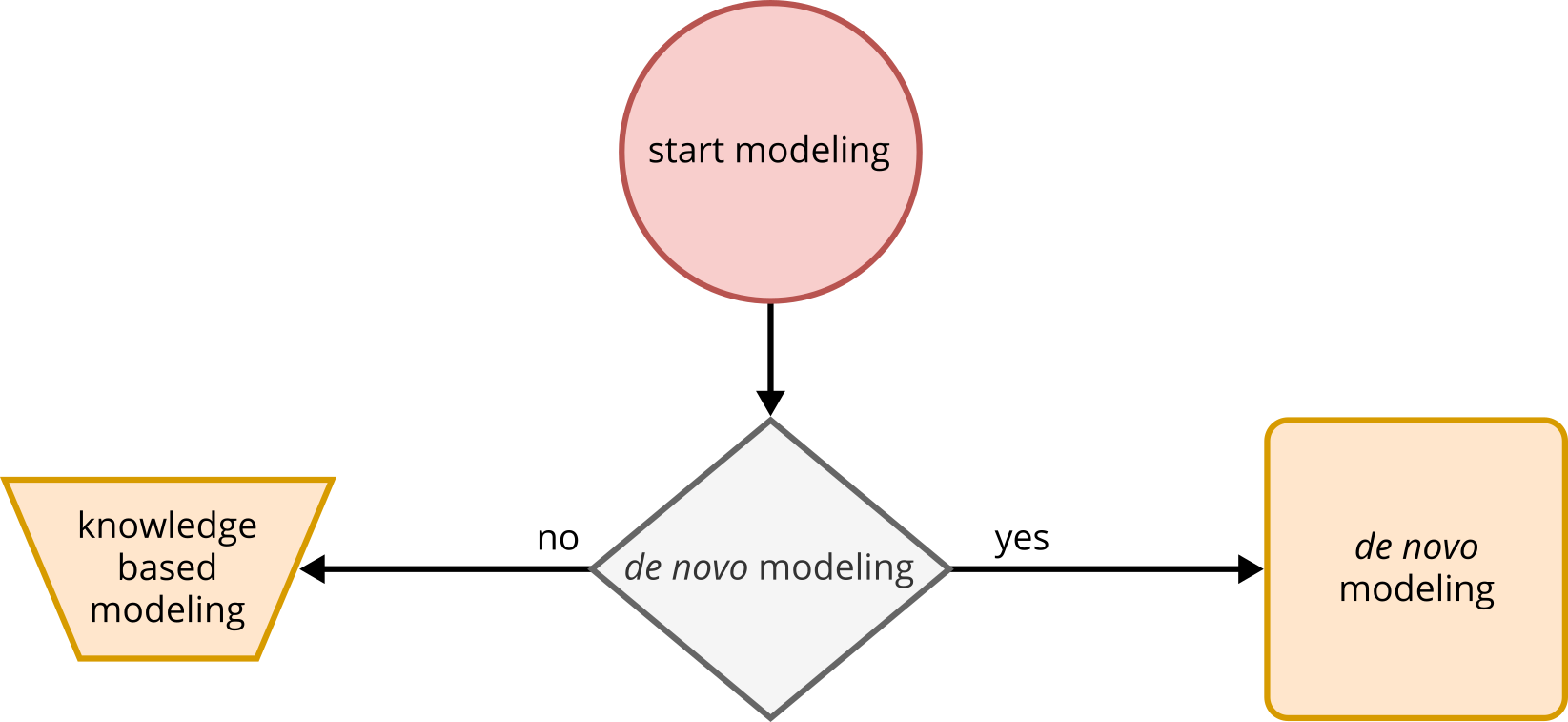
Fig. 3 Starting point of the pipeline. Decision whether to perform de novo or knowledge-based modeling.

When to choose de novo modeling?

• If no existing structures are found in databases.

• If the desired conformation is not available in databases.

• If modeling an ensemble of conformational states.

When to choose knowledge-based modeling?

• If an existing and validated structure model is available in databases.

• If the desired conformational state cannot be modeled using de novo approaches.

• If only small sequence changes need to be made, without significant impact on the structure.

De novo modeling

The de novo modeling pipeline includes three automated processes. The first process uses RNAfold [1] for secondary structure (2D) prediction. Prior installation of this tool is required and can be accessed within the pipeline. An RNA sequence is used as input to initiate the pipeline. The predict_2D_structure() function utilizes a fasta file to predict the 2D structure, saving the result as a text file in the sds_prediction folder. The secondary structure is stored in dot-bracket format, with round brackets “()” denoting canonical base pairings, dots “.” representing free bases, and square brackets “[]” indicating pseudoknots. The resulting file can be edited to modify the 2D structure, such as adding unpredicted pseudoknots.

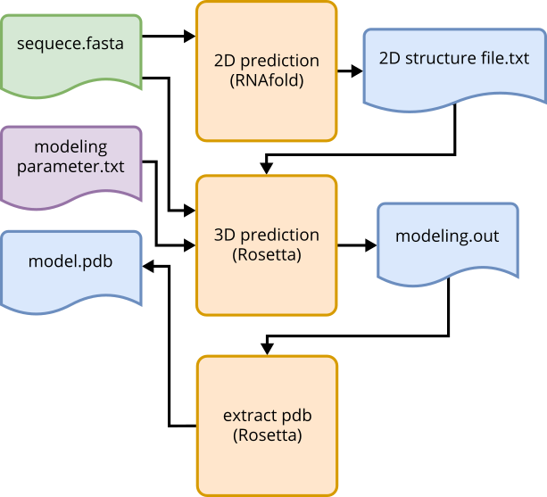
Fig. 4 De novo tertiary structure prediction using RNAFold and Rosetta. Input, output flow using automated methods.

The second process is the prediction of tertiary structure using Rosetta. Prior installation of Rosetta and acquiring a license is necessary. The FARFAR2 [2] extension of Rosetta, activated through rna_denovo, is used for modeling. Inputs include the sequence, the 2D structure, and additional simulation parameters (Parameter: Rosetta). The sequence and 2D structure are automatically extracted from the RNAfold output file. Parameters and results are stored in the rosetta_results folder. The predict_3D_structure() function initiates the modeling by running the submit_jobs.sh bash script. The resulting file is in a Rosetta-specific format with a .out extension. The third process, extract_pdb(), employs the extract_pdb.sh script to generate a PDB file. The PDB structure with the best score, calculated by Rosetta, based on energy calculations of the structure models, is returned. Multiple structure files can also be returned, allowing manual selection of the desired structure model. A general guide for modeling using Rosetta can be found in chapter: Protocol template modeling.

Knowledge-based modeling via PyMOL

The square orange processes primarily use automation, while trapezoidal processes require manual intervention by the user. The purpose of the workflow described here for knowledge-based structure modeling is to demonstrate how existing structures from databases can be modified to create structure models based on knowledge. The tool PyMOL (PyMOL website) can be used for the processes outlined in this workflow. PyMOL must be installed, and a license is required. It is important to have a basic understanding of the desired structure when using this method. This could involve a sequence construct with a known structural core region where structural fragments are missing, or an existing structure where the structural effects of mutations need to be investigated, and so on.

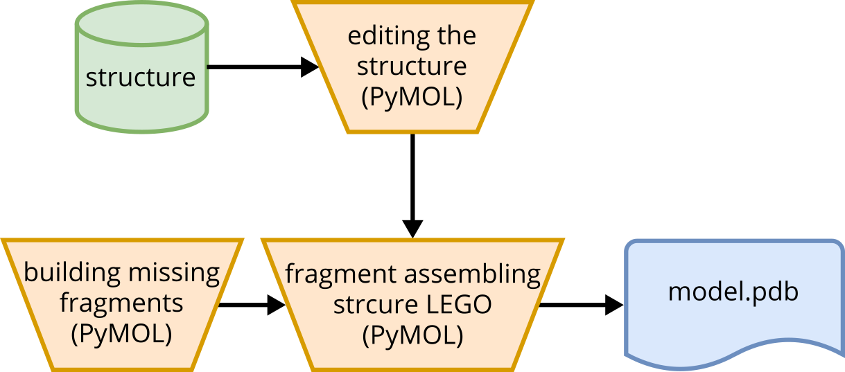
Fig. 5 Conceptual workflow of the non-automated process of knowledge-based modeling using PyMOL.

For example, if an existing structure from a database shows a tertiary contact and should be adapted, it can be processed in PyMOL. A complex structure can be reduced to the tertiary contact, and bases can be mutated to adapt the database structure to an underlying sequence construct. PyMOL provides functionalities such as the Builder tool, which allows mutation and structural adaptations. The Builder tool can also be used to add structural elements or build single-stranded RNA fragments which can be adapted in shape by rotating the backbone of the RNA. Ultimately, the database structure and fragments can be combined and linked using the Builder. This process, referred to as “RNA structure Lego”, involves manual assembly of individual fragments. A detailed guide for this modeling process can be found in the chapter Protocol remodeling structures.

To refine the structure and optimize atomic positions, the simulation software GROMACS can be used for energy minimization through a short molecular dynamics (MD) simulation of approximately 0.5 ns.

While this process is not yet fully automated, it offers the opportunity to generate structural models with maximum flexibility. It can also be used for editing existing models, allowing the incorporation of structural interactions that cannot be predicted by previous modeling tools. Hence, the RNA structural Lego serves as a starting point for adjusting models.

In silico labeling and ACV calculation on static structures

Starting from a structural model, whether knowledge-based or de novo modeled, the structure can now be evaluated for the first time using a calculated FRET value on a static model. To perform this calculation, the programs PyMOL and FRETraj [3] are required. FRETraj must be installed as a PyMOL plug-in to access the FRETraj GUI. The structural model can then be loaded, and user interaction with the program is necessary during this process.

To calculate the accessible contact volume (ACV), dye parameters need to be entered within the GUI. The parameters include the attachment points and the geometry of the dyes, as well as the thickness of the contact volume and the ratio between accessible volume (AV) and contact volume (CV). The attachment points are typically atoms where the dyes are chemically linked, but the choice of atoms is flexible. The dye parameters consist of three radii that define a spheroid, while the linker parameters define a cylinder with specific width and length. These parameters depend on the dimensions of the actual dyes. A detailed explanation of how these parameters are defined can be found in Steffen et al. (2021) [3].

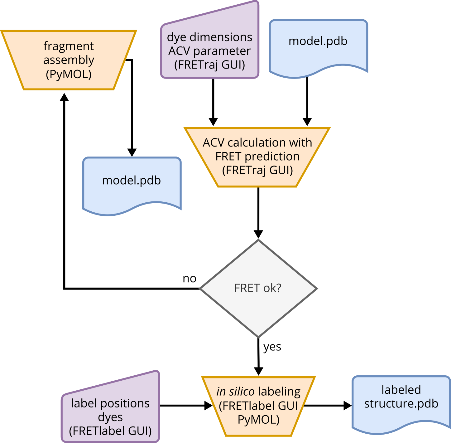
Fig. 6 Guideline for the use of FRETraj in PyMOL and the potential evaluation of initial structural models by FRET.

The thickness of the CV defines the volume around the structure within the accessible volume and the CV fraction can be defined by the ratio of \(r_\infty\) and \(r_0\) from anisotropy experiments [3, 4]. This parameter describes the probability of surface interaction of the dye with the biomolecule. Between two ACVs on a structure, an average FRET value can be determined. The required parameters are the Förster radius \(R_0\) and the number of distances to be measured between single points within the two volumes. The calculation results include the mean distance of the dyes \(R_{DA}\) and their standard deviation \(\sigma\), the FRET value calculated from the mean distance \(E_{DA}\), the distance between the ACV centers \(R_{MP}\), and the distance between the attachment points \(R_{AP}\). The resulting FRET value can be compared to an ensemble FRET experiment or the mean value of an smFRET distribution. The user should qualitatively compare the values, such as, concluding if both values indicate a high or low FRET. Based on the interpretation of the comparison between experimental FRET and predicted FRET, the user can decide whether to remodel the structure or proceed with the model in the next step of the pipeline.

When interpreting the FRET values and the model, it is important to consider that static models do not account for RNA movement. If domain movements are expected, the FRET value predicted here cannot provide a general indication of eventual domain movement in the experiment.

However, this process can assist the designing of experiments. Determining whether a high or low FRET value is present can help in selecting the appropriate labeling position for the experiment [5].

The next step is in silico labeling of the structural model. The tool FRETlabel [4] is used for this purpose, which must be installed as a plug-in in PyMOL to access the FRETlabel GUI. The in silico labeling process involves user interaction with the GUI and is not fully automated. In FRETlabel, the structural model is loaded, and the user defines the dye fragment with its position, chemical method, base, and dye (FRETlabel documentation). The position refers to whether the structure should be labeled internally or terminally. The chemistry category describes the labeling method used to attach the dyes to the attachment points. A base must be selected where the dye should be applied, and the dye can be chosen from a set of predefined options. Once the parameters are defined, the “target residue” can be selected, and the dye can be attached to the model and saved. The in silico labeled structures serve as a basis for MD simulations with explicit dyes.