Data analysis

Creating distance and 𝜅² distributions

To generate a FRET distribution, it is necessary to have a trajectory of dye distances and the orientations between the transition dipole moments of the dyes [3, 8]. This information can be obtained using the two previously created trajectories. One trajectory is used for determining the ACV along the MD trajectory with a constant 𝜅², while the other trajectory directly provides the dye distances and dipole coordinates. In the pipeline, parameters can be defined which include the name of the simulation and the atom IDs of the dye midpoint and dipole atoms.

Determining distance and 𝜅² from ACV calculation:

The first step involves loading the trajectory using mdtraj, which requires the xtc and pdb files of the trajectory. The parameters necessary for the ACV calculation is shown here. Additionally, the atom IDs of the attachment points, which can be extracted from the PDB file, need to be specified. Utilizing the defined dye parameters and the parsed trajectory, the ACV can be computed using the fretraj.cloud.pipeline_frames() function. It is crucial to specify the desired calculation step width. For instance, in a 1 µs simulation, it is recommended to calculate one ACV per 100 ps. However, it should be noted that an increased number of ACVs will result in longer calculation times. The trajectory can be saved using fretraj.cloud.save_obj(). The fretraj.cloud.Trajectory() function generates a trajectory of average dye distances based on the ACV’s and a 𝜅² value of 0.66 is assumed. This trajectory file is saved as r_kappa.dat in the MACV directory.

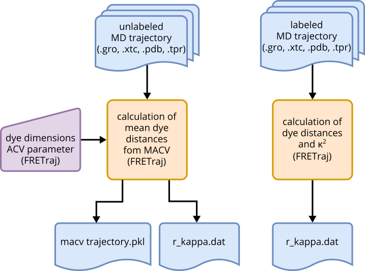
Fig. 8 Methods for generating distance-𝜅² trajectories.

Determining the distance and 𝜅² values from explicit dye simulations

To generate the 𝜅²-distance files, the dye dipoles must be defined. This requires finding the atom IDs of the dipole atoms and the central carbon atom of the dyes, which can be obtained from the gro file of the trajectory. Using these atom IDs and the MDAnalysis package, the spatial coordinates of the atoms can be extracted from the trajectory. The function get_rkappa_file_from_dyes() can then calculate the 𝜅² values based on these dipole coordinates and the distance between the central carbon atoms of the dyes. Only the atom coordinates need to be provided. The calculated data is saved in a file named r_kappa.dat, which can be subsequently utilized by the FRETraj Burst module.

Burst calculations and data visualizations

Once the distance and 𝜅² trajectories have been generated, they can be processed using the Burst submodule of FRETtraj. This submodule allows for simulating long-time FRET experiments on MD trajectories of a microsecond timescale by sampling photon events. Several parameters need to be defined, which are categorized into Dyes, Sampling, FRET, Species, and Burst (Burst Parameter).

In the Dyes category, experimental properties of the dyes and the experimental setup are defined, such as lifetime, quantum yield and detection efficiency. While these values cannot be obtained from the simulation, they are necessary for calculations of photophysical parameters like the anisotropy or FRET.

The Sampling category defines parameters related to the burst simulation, including the number of bursts to be simulated, frames to skip at the beginning and end of the trajectory, and whether multiprocessing should be used for calculations.

The Species category allows for defining different groups of structures within an ensemble. Each species can be given a name, and the corresponding dipole coordinate files and r_kappa.dat files can be specified. Additionally, a probability can be assigned to each species, and multiple species can be defined using lists.

In the Burst category, the burst itself is defined. This includes specifying a burst size distribution using a Poisson distribution with upper and lower limits, as well as a lambda value (\(\lambda\) = -2.3). The burst size distribution can also be obtained through experimental measurements and imported as a file with the option burst_size_file. Averaging can be performed within each species or across the entire ensemble.

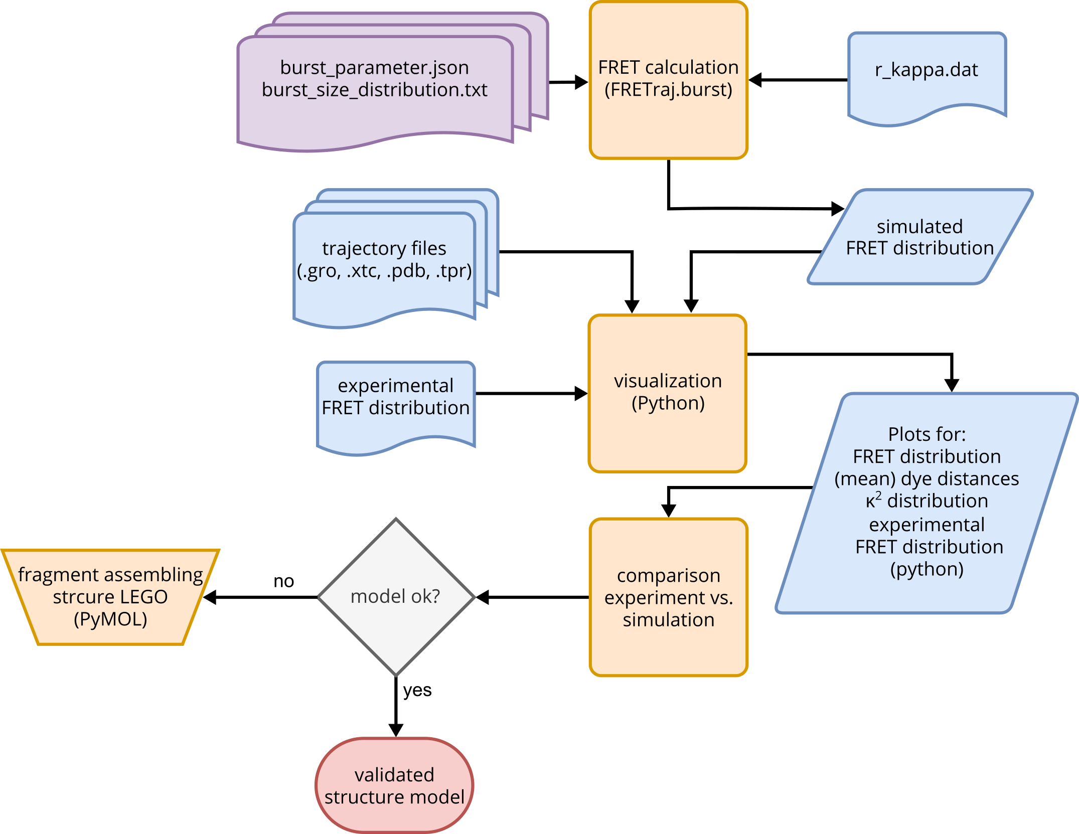
Fig. 9 Workflow for the simulation of FRET experiments from the distance-\(\kappa^2\)

With the above defined parameters, FRET distributions can be simulated using the fretraj.burst.Experiment(parameter) function, applicable to both MACV and explicit dye simulations. The resulting FRET distributions can be compared with each other. Functions have been developed to facilitate visualization of the calculated data. This includes comparing simulated FRET distributions from MD and MACV with experimental data, plotting histograms of dye distances calculated from MACV and explicit dye simulations, and generating trajectory histogram plots.

For MACV, the FRET efficiency can be plotted without sampling and compared with the initial FRET value of the static model before simulation, demonstrating the influence of RNA movement on the FRET efficiency. Finally, the dynamic structural model should be compared by the user with experimental data, and the quality of the model in relation to the experiment is subject to user interpretation. If the model does not match the experiment, a feedback loop can lead back to the knowledge-based modeling approach with PyMOL.